Category Archives: tutorials

Drawing linguistic structure trees

The LaTeX way

I use LaTeX to make my trees—the qtree package for simple trees, and xyling for anything more complicated like prosodic structures, Hasse diagrams, etc. For detailed instructions and links, see the LyX Wiki for Linguists. This page explains not only how to do syntax trees but also how to draw moraic structures, how to include IPA in a syntax tree, and so on.

Standalone applications

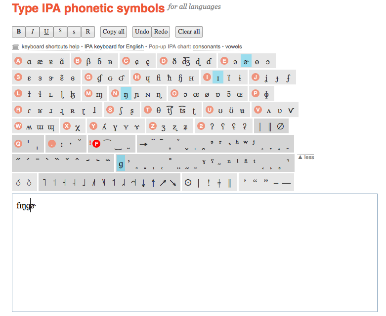
There are several standalone programs, both webapps and desktop apps, that you can use to enter tree structures, and they will render the structures as pictures for you. I like  phpSyntaxTree: Given the input [S [NP [N Trees]] [VP [V grow] [PP in apps]]], this produces a PDF with the following image.

php syntax tree demo


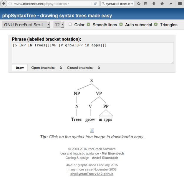
It also supports Unicode now so you can use IPA in your trees as well as have math symbols in your labels.

For desktop apps specific to your OS, do a search–there is definitely stuff out there for Windows and Macs, although there may no longer be support for the apps because they tend to be a labor of love sort of thing.

The Fingerpainting Method
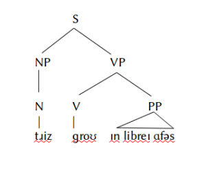
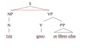
In Libre Office, Microsoft Office, and no doubt other programs, you can draw the trees by tabbing the words into position and adding the lines using the line drawing tool. Here is what I got when I did this in Libre Office. (In order to make it look like that, I had to individually right-click on every line and change the color to black, because it defaults to blue and I couldn’t stand that and I could not be assed to figure out where the defaults are.) So, as you can see, the method is slow and ugly, but it has some benefits.

libre office line drawn tree

  1. It works when you do not have an internet connection.
  2. The tree is entirely contained in your document and uses the same fonts as your text, so even though you get an ugly tree, the fonts match
  3. There is no need to worry about embedding fonts in your PDF file, unlike the Arboreal method (next).
  4. You do not have to learn even the rudimentary bracketing syntax that phpSyntaxTree and others require, so if you are really afraid of any sort of structure and notations, this method is for you. Then again, if you are this afraid of structure, you should probably give up because linguistics might not be for you.
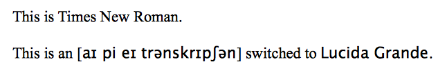
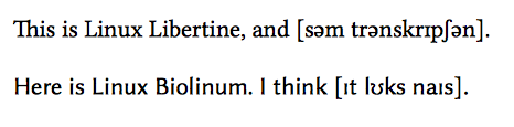
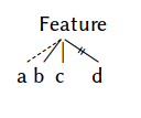


Arboreal and Moraic

This is an old approach to drawing trees. You tab or space your words into position and switch to the font, which provides characters that look like lines at different angles. There’s a triangle or two. The output looks more consistent than the fingerpainting method above. Notice that the screenshot on the right has the red spellchecker underline–it’s because the lines are actually characters, and the LibreOffice spellchecker treats them as (ill-formed) text. The red lines would not be visible in the PDF.


This method has many downsides, however.

  1. The fonts are proprietary and cost $20 each.
  2. These predate Unicode so modern computers don’t know what to do with them unless they have been converted to pictures first. So these fonts need to be explicitly embedded in the PDF or else they render as capital Gs, etc.
  3. The limitations of the characters restrict what types of trees you can draw—for example, the triangles only come in a few sizes.
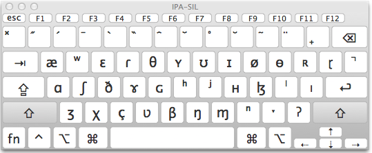
  4. I spent about 10 minutes henpecking around the keyboard looking for the right characters to show you, and the font kept switching back to the default text font. The key map on my OS did not even know how to render these characters, so I was flying blind.


Comments Off on Drawing linguistic structure trees

Filed under international phonetic alphabet, trees, tutorials

International Phonetic Alphabet fonts and keyboards

Introduction

This page explains how to set up International Phonetic Alphabet IPA fonts and keyboard layouts on your computer.

Keyboard layouts allow you to enter IPA fonts directly by hitting key combinations, as explained below. I work with the IPA a lot, so I find  keyboard entry indispensable.

Which font to get?

  • Most modern computers should already have some fonts that can display IPA characters. But what you sometimes see is some characters appearing in a different font than the rest of the text, like this:

lucida_grande_switch

  • This is because many fonts only have a partial Unicode character set, which covers the standard (Latin alphabet) ASCII set but not much more. Your computer will substitute a more comprehensive font if its default font lacks the IPA characters. On Mac OS, this is Lucida Grande, for example.
  • I like Linux Libertine and Linux Biolinum. The fonts are freely distributed under a GNU Public License, and they work on any OS.

libertine

  • Another popular font is Doulos SIL. See the SIL webpage for details. I think it’s kind of ugly.

How to use the fonts: Web interface

  • This is the slow but universal way. It even works on iOS and Android.
  • Go to ipa.typeit.org. You can point and click on any IPA symbol with your mouse or finger, and the character will appear in the text box.
  • From there, you can copy and paste the transcriptions into your document writing program, then change the font of the doc to Linux Libertine if you like, and you’re done.

IPAtypeit

OS-specific Methods

These are much faster and more efficient. Invest some time into learning them and you will save yourself time in the long run.

Windows

  • Check out this page, ipa4linguists. It explains how to use the Character Map, and also covers the various quirks of Windows.
  • I found one IPA keyboard layout for Windows. I cannot vouch for this thing, but if it works, that is by far the most efficient way of working with IPA fonts (see the next section on Macs).

Mac OS

The IPA-SIL keyboard layout

  • These instructions should be current as of Mac OS 10.8x and 10.9x.
  • I use the IPA-SIL keyboard layout, which I am providing it for download here since SIL is no longer distributing or supporting it. The zip file includes a PDF with more detailed documentation.
  • The keyboard layout allows you to type in IPA without using “dead keys” (keystroke sequences that turn into a single character, for example, typing “i” and then “=” gives you “ɪ”). Ain’t nobody got time for that.
  • Here is the workflow:
    • hitting Cmd+Space switches the input method from English to IPA-SIL.
    • Once in IPA-SIL mode, you can type normal lowercase Latin characters without doing anything.
    • If you press the Shift key while typing s, i, f, d, t, q, n, you get  ʃ, ɪ, ɤ, ɾ, ð, θ, æ, ŋ respectively (The keyboard map shows you which keys do what, though you do not need to use the keyboard map to enter the keys):
What your keyboard will type in IPA-SIL when "Shift" is depressed

What your keyboard will type in IPA-SIL when “Shift” is depressed

  • Pressing Alt+Shift accesses these:
Alt+Shift on the IPA-SIL keyboard layout

Alt+Shift on the IPA-SIL keyboard layout

  • And Alt alone accesses these:

Alt on the IPA-SIL keyboard

  • For anything else, you can use the Character Viewer on Mac OS. Just open it from your Input Methods menu (which can be enabled from Settings>Keyboard).

Installing the IPA-SIL Keyboard

  • There are more detailed instructions in the PDF inside the zip file linked above.
  • The basic procedure is:
    • put the IPA-SIL.keylayout file into Users/yourusername/Library/Keyboard Layouts. Put the IPA-SILicns icon file there as well.
    • then enable the IPA-SIL keyboard by going to Settings>Language & Text > Input sources. Scroll down the long list of keyboards until you see IPA-SIL; if you don’t see it, you might need to restart the machine. Then check it.
    • Check on “Show input menu in menu bar”.
  •  Mac OS likes to take away features, especially ones that allow you to customize the system. If you cannot see the Library folder inside your Users/yourusername directory, go to your favorite search engine and look for the solution that is specific to your version of Mac OS.

Linux

  • The only method I was able to get going on Linux is ipa-x-sampa. It’s reasonably user-friendly and does not require a million steps that result in failure, like SIL’s Keyman thing. In order to use ipa-x-sampa, you need to enable IBus, and then
    apt install ibus-table-ipa-x-sampa

    If that fails, there is also Character Map type thing that you can use.

  • For some non-IPA characters that linguists use, it was suprisingly difficult to figure out how to enter them on Linux. The crucial bit (on Linux Mint, anyway, but probably others too) is to enable a “Compose Key” in your keyboard layout. Go to Preferences>Keyboard>Layouts, select “English (US)”, then Options, then find “Position of Compose Key”. I chose Caps Lock for mine. What this does is allow you to type various characters like é and ü by pressing the Compose Key together with ‘ or “, etc. A list of all the default key combinations enabled in Linux can be downloaded as a tab-separated text file here.

iOS and Android

  • Go to your “App store” or whatever and search for “IPA keyboard”, or “IPA phonetics”.

Comments Off on International Phonetic Alphabet fonts and keyboards

Filed under international phonetic alphabet, tutorials

Praat tutorial


Introduction

  • Praat is a freely available program written by Paul Boersma and David Weenink.
  • It is primarily intended for acoustic analysis of speech, but it has some additional functions such as speech synthesis and some constraint-based grammar learners. It can even run some basic perceptual experiments.
  • The program is very powerful and has many features, with new ones being added all the time. There are only a few features that a beginning phonetician would need; this tutorial covers them.

Installing Praat

  • Go to http://www.fon.hum.uva.nl/praat/ and follow the instructions for your operating system.
  • Mac users–drag the Praat.app file into your Applications folder. You may then add a link to the program onto your dock so you can enjoy looking at this icon every day. [EDIT 2020/2021: it is with great sadness that I learned that Praat authors finally changed the icon. It still has a mouth and an ear, though. I am keeping this here for historical reasons. It’s too important.]
Praat
  • Not enough space on your disk? This is an issue that Chrome OS users sometimes report. (Chrome OS stores everything in the cloud so the machines often have very little physical storage.)
    • Try to free up space on your machine. I would start with your browser’s data, which can be huge.
    • Chrome OS runs Praat inside a Linux installation, which you might already have. If not, see the instructions here for how to do it.
    • My Linux installation of Praat is 25MB, plus another 25 for the no-GUI version (my installation is on Linux Mint, not inside Chrome OS, so your mileage might vary).

Praat basics

The two windows

  • When you open Praat, two windows appear: the Objects window and the Picture window. You won’t need the Picture window most of the time, so close it. We’ll come back to it at the end of this tutorial.
  • The Objects window starts out empty, but once you open sound files and manipulate them, it will contain sounds, spectrograms, text grids and any other objects that you work with:
The Praat object window on a Mac.
  • Important: the objects in the Object window are temporary and only exist in Praat’s working memory. If you change the content of an audio file using Praat, it won’t automatically save the changes. If you try quitting without saving the objects, Praat will prompt you to do so.

Opening, playing, recording, and editing audio files in Praat

Opening an existing sound file

  • Open Praat, click on “Open”, then “Read from file”. You will see a “Sound” object appear in the window, which you can then “View and Edit”.
  • In Mac OS, you can also drag your audio file or files onto the Praat icon. All of the files will then appear as sound objects in the list at once. See if your OS supports drag-and-drop opening of files.
  • Depending on the length of the recording, you will see either the waveform with an empty window below it or a waveform above the spectrogram.

Converting stereo to mono

  • If you are seeing two waveforms, your file is in stereo (was recorded with two microphones):
stereo_waveform
The two lines of black squiggles labeled “Channel 1” and “Channel 2” are your two stereo channels.
mono_waveform
Here, we extracted just one channel (the top one, recorded with the “left” microphone). Now we have a mono sound.
  • For speech analysis, you do not need stereo, since the vast majority of humans have only one mouth.
  • To get a mono file, you can extract one of the audio channels, like this:
  1. Return to the Objects window.
  2. Select the stereo Sound object.
  3. Click on “Convert”.
  4. Select “Extract one channel”. Unless the two channels are really different from each other, you can just accept the default, “1/left” channel.
  5. The new object will have the same name as the old but with “_ch1” appended at the end. Don’t forget to save it if you want to use it again.

Recording an audio file right into Praat

  • You can record right into Praat, as long as your computer has a built-in microphone. Most likely the recording will not be of awesome quality, but it’s fine for practicing with the program.
  • To record a sound, click on “New>Record Mono Sound”, and hit “Record” in the window that opens. You can accept all the defaults in that window.
  • One tip about recording: if you are using your laptop, you might not know exactly where the microphone is on it. I have no idea where the mic is on my laptop, actually. I just leaned in and talked close to the laptop. Here is the resulting recording of me saying a sentence in Russian, [napʲisənə lʲdotʲexnʲikə pʲatʲ ras] “The word ‘ice technology’ is written five times.”
ljdotexnika_me
A waveform and spectrogram of a sentence I recorded straight into my MacBook Air using Praat.

Recording: a note about clipping

  • When you record audio for speech analysis, you want the signal to be as loud as possible without exceeding the range of your microphone’s sensitivity.
  • Look at the black number in the upper left-hand corner of the screen, next to the waveform. Your recording should get as close to 1 as possible, but the waveform should not protrude above it. If the amplitude of the recording exceeds the range of the microphone, you get clipping.
  • A clipped recording is missing parts of the signal, and it sounds awful. Avoid.
  • Here is what clipping looks and sounds like. I had to pretty much yell at my laptop to get this to happen, so you’ve been warned. Your Praat recording widget has a meter display that stays green while you’re in good range and turns red when you are in the clipping range.
The last "clipping" is clipped. See how the waveform extends outside the waveform window?
The last “clipping” is clipped. See how the waveform extends outside the waveform window?

Playing audio

  • Once you have a Sound object, you could just hit “Play”. Usually, we want to play only portions of a file, sometimes repeatedly as we try to transcribe or determine the boundaries of a segment.
  • To play portions of a file, click on “View & Edit”, and make a selection with your mouse.
  • The playback options are in the “View” menu. Yep. I actually had to look for this just now because I usually play back the selection using the Tab key. Tab will also stop playback. Shift+Tab plays the visible window.
  • For Mac users: I’ve used a Mac for over a decade now but I still cannot keep track of the little symbols that apps use for keys. Here is a reference.

Editing a file

  • There are many things you can do to edit a file. Perhaps the most basic function, and one that you might find useful long after this class ends, is to cut out parts of a file.
  • First, open the Sound object of your file in the View & Edit window.
  • Make a selection you want to keep, using the mouse.
  • If you want to make a really neat cut, you can “Move start of selection to nearest zero crossing”–this is an option at the bottom of the “Select” menu. Then do the same for the end of the selection. What this will do is adjust the selection so that it starts and ends with a silence (zero amplitude).
  • Then click on “File”, and you have several options here.
    • You can put the selected sound into its own sound object, if you want to keep doing things to it (“Extract selected sound”, either preserving the time markings from the original file or resetting them to zero seconds).
    • You can also save the file to disk. There is a range of options, but a .WAV extension is the basic one.
  • The options above do not alter the original file or the Sound object in Praat’s memory.
  • If you want to modify the Sound object or the file, you can cut a portion of it out–useful if you have a long period of silence, or if you want to make someone say “got” instead of “Scott” or whatever. This is done via “Edit>Cut”.
  • Once you cut a portion out, it is placed on your clipboard (computer’s working memory); if you then save the Sound object to the original file again, the file will be permanently altered. If you do not want that, save it under a new name instead.
  • You’ll see other options in the menus, which are more or less self-explanatory. Feel free to play around with them, and remember that nothing is permanent until you save to disk.

Viewing spectrograms, pitch tracks, formants

  • Praat can only display spectrograms for relatively small chunks of audio, so if you want to see a spectrogram for a word, zoom in on it.
  • You can select a part of the recording with the mouse, and then use the View menu to zoom to that selection. The View menu is fairly self-explanatory.
  • There are keyboard shortcut hints in the View menu and many other places in Praat! Use them. I use Cmd+N to view the selections on Mac OS.
  • Here is a waveform and a spectrogram of a female Russian speaker (not me) saying [napʲisənə lʲdotʲexnʲikə pʲatʲ ras] “The word “ice technology” is written five times.” This sentence is a bit over 2 seconds long.
ljdotexnika_spectrogram
A waveform and a spectrogram of a 2-second Russian sentence.

Making a spectrogram look good

  • If you are working with a fresh install of Praat, your spectrograms most likely will look a lot more gray than the ones you see above. This is because the dynamic range is set very high in Praat by default–at 70 db. You want something like 30-50 for a recording that has some background noise.
  • The obligatory metaphor: Dynamic range refers to how low the cut-off is for the volume of frequencies that the spectrogram visualizes. The lower the number, the less you see. Think of it as taking pond water out of a bucket. The deeper you dip, the more muck you’ll scoop up. If your pond (=recording) is very clean, then you can dip pretty low (i.e., have a high number dynamic range). If your pond is mucky and dirty, then you better skim from the top (i.e., have a low number in your dynamic range).
  • Of course, just because you are skimming from the top doesn’t mean you have clean water. Here is what the laptop audio I recorded looks like with the defaults. You can clearly see two bands of air conditioner noise, the lower of which is around 2400 Hz. This kind of noise really interferes with acoustic analysis of speech:
The same recording of me saying that "ice technology" sentence, with a default dynamic range of 70 db. The two bands of noise are from the air conditioner in the background.
The same recording of me saying that “ice technology” sentence, with a default dynamic range of 70 db. The two bands of noise are from the air conditioner in the background.
  • To set the dynamic range, click on “Spectrum>Spectrogram settings”. Change it in 5 db increments until it looks good.
  • You can also change how high the frequencies go in the spectrogram display. The default is 0-5000 Hz. You can expand it quite a bit–some fricatives have noise at frequencies above 12000 Hz.

Viewing pitch tracks, intensity, and formants

  • Pitch.
    • This is pretty simple. While you have the Sound object open, click on “Pitch>Show pitch”. You will see a curvy blue line appear in the spectrogram window.
    • In Pitch Settings, click on “drawing method” and select “speckles”. I think it looks better than Praat’s default, “automatic”.
  • Intensity.
    • Click on “Intensity>Show intensity”. A yellow line will appear in the spectrogram window.
  • Formants.
    • Praat can also show you formants, and you can probably figure out the procedure for those on your own.
    • There is one thing you will have to change in the Formant settings depending on whether you are looking at a male or female voice: the maximum formant should be set for 5500 Hz for female speakers, and 5000 Hz for male ones.
    • These formant dots are estimated by Praat; you cannot always trust them.
  • Pulses.
    • This method visualizes glottal pulses that show up in voicing. If you turn “view pulses” on, you’ll see vertical blue lines wherever Praat thinks the glottal pulses occur.
  • Here is the Russian word [bʲitonəmʲiʂalkə] ‘concrete mixer’ with the pitch track, intensity, formants, and pulses turned on. You would rarely need to see all of these things at once, this is just for demonstration.
betonomeshalka
Pitch track: blue line, intensity: yellow line/green numbers, formants: red dots, glottal pulses: blue vertical lines in the waveform window.

Annotating an audio file with TextGrids

  • A TextGrid object allows you to mark certain periods or time points in a sound file.
  • You can have several tiers in a TextGrid: one to mark word boundaries, another to mark consonants, vowels, whatever you want.
  • You can type into the TextGrid using IPA fonts. See this page for more information on how to set up your computer so that you can do this painlessly and quickly.
  • Praat distinguishes between “point tiers” and interval tiers.
  • To create a TextGrid, start from the Objects window. Select your sound object and click on the “Annotate” button to the right.
  • You’ll see this window. Why the program suggests “Mary John bell” as the default tier names is a mystery to me.
Default TextGrid dialog
  • You can either name all your tiers at once, as shown here, or name the first one and add more later.
  • I named my three tiers “word, segments, vowels”–you see them in the screenshot below.
  • Now comes one of the Praat gotchas: “View & edit with sound” is highlighted, and you would think that this would allow you to view your sound file and edit the TextGrid at the same time, but no. Clicking on that button just tells you that in order to do what you want to do, you have to select both the sound and the TextGrid in the objects window and click on the “View & Edit” button.
  • You can select the TextGrid and Sound objects with the mouse or with your keyboard keys. On a Mac, Shift + arrow (up, down) will let you select two adjacent objects in the window.
  • If you have more than one object in the list, make sure you select the TextGrid that goes with your sound file!
  • Once you are in TextGrid edit mode, you can add text on tiers, copy interval boundaries from one tier to another, and navigate between tiers and between intervals using either the mouse or just your keyboard–make sure to poke around the “Select”, “Interval”, and “Boundary” menus to see all the options.
textgrid
A TextGrid with three interval tiers, labeled in the International Phonetic Alphabet.
  • Make sure you save your TextGrid when you are done. By default, the TextGrid will be given the same name as your sound file, and the extension is .TextGrid.
  • Advanced note for the computationally curious: open a TextGrid in a text editor such as TextWrangler, and you’ll see that it’s just a Unicode text file with detailed information about the time points when a tier begins and ends, and its label and type. It looks like this:
File type = "ooTextFile"
Object class = "TextGrid"

xmin = 0 
xmax = 1.2121237048836804 
tiers? <exists> 
size = 3 
item []: 
    item [1]:
        class = "IntervalTier" 
        name = "word" 
        xmin = 0 
        xmax = 1.2121237048836804 
        intervals: size = 2 
        intervals [1]:
            xmin = 0 
            xmax = 1.1468403366828597 
            text = "bʲitonəmʲiʂalkə" 
        intervals [2]:
            xmin = 1.1468403366828597 
            xmax = 1.2121237048836804 
            text = "" 
  • Can you guess what “xmin” and “xmax” refer to, and how you might collect information about interval duration automatically by script? More on that below.

That Picture window

  • Finally, we get to the mysterious Picture window. The point of the Picture window is to make professional, publication-quality images from your spectrograms, waveforms, and whatever other aspect of speech that you use Praat to visualize.
  • Whenever you see a “Draw” or “Paint” option associated with an object, it refers to the Picture window.
  • For example, open a sound file and click on the Spectrum menu–you’ll see “Paint visible spectrogram” as an option. The same “paint” option is available for intensity, pitch, formants, and other views.
  • To make a spectrogram picture with a pitch track overlaid on top, I “painted the visible spectrogram” and then “painted the visible pitch” while unchecking the “erase first” box. This superimposes the pitch track on top of the spectrogram picture.
  • Poke around the menus, check out the options, and see what “Garnish” does.
picture_window_editing
Screen shot of the picture window in action
betonomeshalka
A nice picture of the word [bʲitonəmʲiʂalkə], with a speckled pitch track superimposed in black.

Beyond basics

  • To get a sense of the full power of this program, you can just look at the various collections of Praat scripts that people have made available.
  • Praat uses its own scripting language, which is based on the commands in the program’s menus.
  • You can automate a lot of tasks:
    • Record a word list, cut it up into smaller files at silences automatically and label all the smaller files from a text file you specify.
    • Normalize the intensity of a bunch of different audio files, so they all sound approximately equally loud
    • If you have to label a lot of audio files, you can automate opening and TextGrid creation.
    • You can also automate the collection of durations, intensities/pitch at various time points, Praat-estimated formant values, and so on.
  • To get a sense of all the options, do a web search for “Praat scripts”. I really like Mietta Lennes’ page, but there are many others, such as this Google Sites archive.
  • There is also the actual Praat Help, which you can search.

Comments Off on Praat tutorial

September 3, 2016 · 14:53

Running R on multiple cores, Mac OS

If you do something computationally intensive, such as fitting a hierarchical/mixed effects model with random slopes in the lme4 package, you might find that R takes hours and sometimes even days just to tell you that it didn’t converge. In my struggles with R, I figured out this way to run several models at a time on several CPU cores. Here is how I did it.

When invoked from R.app, R runs on just one CPU at a time in Mac OS. But if you run R from the command line, you can assign different R processes to different cores:

  1. Open Terminal. (Macintosh HD>Applications>Utilities>Terminal.app).
  2. Start screen by typing screen at the command prompt.
  3. Start R by typing R at the command prompt on the screen emulated terminal. You might have to hit space to get to the prompt itself–check the screen manual for more.
  4. Paste in your R commands from wherever you keep them. Alternatively, run an R script using the source() command. Here’s a small example:
  5. setwd("/blah/blah/blah/place_you_want_your_output/")
    exp = read.csv("your_dataframe.csv") #Make sure it's in the working directory
    library(lme4)
    Sys.time() #this tells you when R started running the model
    model1<-lmer(blah blah); Sys.time(); save(model1, file = "model1.Rda") #this is your huge fully crossed model.

  6. Since R can take a while to fit an lmer model (I've had models run for 91 hours before failing to converge!), you might want to let R run in the background while you are doing other things. Running R in screen allows you to do that. Disconnect from the screen while R is running by hitting Ctrl+A and then Ctrl+D.
  7. You can reconnect to the R screen by entering screen -R at the command line.


(These instructions were current as of R 2.14 on Mac OS 10.6.8, and my iMac has a 3.06 GHz Intel Core i3 processor and 4 GB of 1333 MHz of RAM. If you know that something has changed, please tell me!)

Once your .Rda file is saved, you can open it in R to inspect the model using summary(model1). If you get a message about non-convergence, use the model you did get to decide which random slopes to remove. Here is how to decide:


sort(sapply(ranef(model1)$subject, sd))
sort(sapply(ranef(model1)$word, sd))


Take the random effect term with smallest standard deviation out of the model and try running the model again.

Since there is a chance that your next model won't converge, either, you can run multiple instances of R on the same Mac by repeating the steps in 1-6 for different models. When you run the screen -R command, you'll see that you have multiple screens running; connect to each of them separately by using the screen ID number you see.

You can of course connect to your Mac remotely using SSH and connect to the R-running screens to check on whether the models are still running, or use top to check how much CPU % your various instances of R are using.

Comments Off on Running R on multiple cores, Mac OS

Filed under R, tutorials

Switching to LyX for Linguists

Introduction

This page explains how users of OpenOffice, Microsoft Office and other word processors can migrate to LyX, a Graphical User Interface for LaTeX.

I rarely use anything other than LyX these days for work, but you should be warned that switching to LyX/LaTeX is not a dabble, it’s a commitment. This page will get you started, but to really learn and understand how it all works, you will definitely have to poke around the manuals and have to decipher unclear instructions on your own. This is the price you pay for free software.

Advantages of LyX

  • Free
  • Stable
  • Fast
  • Compact: takes up very little room on your computer (11 times smaller than MS Office) and produces small files
  • Produces beautifully typeset PDF files that are readable on any machine
  • Makes typesetting equations and mathematical formulas easy
  • Excellent, powerful bibliography support
  • Easier to learn than LaTeX, since it is almost a WYSIWYG environment (i.e., what you see on the screen while you are editing the document looks almost like the final output)
  • Can export to HTML and to LaTeX
  • Better suited to the needs of linguists than OpenOffice. LyX even includes a special Linguistics module.

Disadvantages of LyX

  • Steeper learning curve than for word processors
  • Some things that are very easy in MSWord are harder in LyX, e.g., trees and some features of tables (beats OpenOffice, though!)
  • This is an open-source program, so occasional bugs are introduced after updates, even as other bugs are fixed
  • Many of the things linguists need to do require special packages that you have to download; the packages themselves require learning
  • Many of the more advanced typographic tasks require using the LaTeX mark-up language, so you do not know what your document will look like until you typeset it.
  • You have to pay very careful attention to the syntax of LaTeX code. Just as in HTML, misplaced spaces, brackets, and slashes can break your file
  • If you collaborate with MS Word users, you have to get MS Word or Open Office; LyX documents do not easily convert to those formats
  • It only does the one thing–make documents. For your spreadsheet and slide presentations, you have to keep Open Office around

Downloading and setting up LyX

  1. Since LyX is basically a sophisticated front end for LaTeX, the first step is to get a working LaTeX installation.
  2. Mac: Install MacTeX. MacTeX is a large download because it includes several programs. But, it puts everything on your computer where it is supposed to go, including BibDesk and a spellchecker program (which I usually delete after installing).
  3. Windows: get MikTeX.
  4. Linux: you might already have both LaTeX and LyX on your system; it ships with some distributions. If not, apt-get install lyx should do it (it also installs the prerequisite, Tex Live, which uses up a ton of room and takes some time to download).
  5. Download LyX here. To check whether it works, open one of the Help manuals that comes with the program and make it into a PDF file. Here’s how:
  6. Open the LyX program, and go to Help>Tutorial.
  7. While the Tutorial is open, go to View>PDF(ps2pdf). If everything is installed correctly, you should see a PDF file of the Tutorial shortly. Otherwise, you’ll get a (possibly very) cryptic error message, and then God help you.
  8. Get a bibliography program. If you are a Mac user, you should have gotten BibDesk as part of MacTeX. Alternatively, get JabRef, which runs on any platform. JabRef is a freely available Java-based program that is similar to Endnote. Once you set up this program, you will be able to edit your bibliography database and search for references. If I were you, I would borrow someone else’s BiBTeX file. Of course, if you’re the strong silent type, you can also make your own from scratch. Note: The most recent distribution of LaTeX that I have came with a spellchecker program, Excalibur. LyX uses aspell and ispell, which I think are older LaTeX spellcheckers. I get annoyed with spellcheckers, but if you like them, perhaps you can figure out how to use them and tell me whether they are any good.
  9. The next step is to create and populate a texmf directory, which is where you keep extra packages (extensions not normally included in a TeX distribution). You’ll need them to do special formatting, like dashed lines in tables and so on.
    1. Mac: Re-create the following structure on your machine. You can look inside my texmf directory for reference.
      Macintosh HD/Users/YourUserName/Library/texmf/bibtex/bib/... (your bibliography files, with the extension .bib, go here)
      Macintosh HD/Users/YourUserName/Library/texmf/bibtex/bst/... (your custom bibliography formatting styles, with the extension .bst, go here)
      Macintosh HD/Users/YourUserName/Library/texmf/tex/latex/... (your latex packages go inside this directory. They can be inside other folders)
      Shortcut: you can simply take my texmf file and unzip it into your Library folder. If you do not see a Library folder, it is probably hidden, so you need to modify your OS view settings for these folders (find out how to do this for your version of Mac OS). Reconfigure LyX afterwards (LyX>Reconfigure), and it should find all the packages you have installed on your machine. You can verify that it did so correctly by going to the Tools>TeX Information menu of LyX and looking at the paths of installed .bst and .sty files. If new things aren’t showing up, hit “Rescan”. You can get additional packages from CTAN. Check CTAN for package manuals, since NONE of them are self-explanatory.
    2. Linux: As for Mac, re-create the texmf/tex/latex/etc. tree inside your user directory. Where to put it: you can get away with ~/texmf, but also see here for more complicated setups: http://math.arizona.edu/support/tex/accountpackages.html. As for Mac above, Reconfigure LyX (LyX>Tools>Reconfigure).
    3. Windows: It appears that there is no standard location for the texmf folder on this OS. You can put it wherever you want, but you will need to go through the extra step of registering it with MikTeX. Moreover, apparently, nothing happens automatically on a Windows LaTeX installation, so you have to update every time you add a package. Here are the instructions (see here for the full story):
      1. Run the MiKTeX “Settings” application (from the Start menu) and go to the “Roots” tab. That lists the directories on the search path MiKTeX uses. Add the location of your texmf folder to that tab (Add… button) and move it up to the top of the search chain.
      2. Whenever you add something to your local texmf directory, they should run the Settings application, and on the General tab click “Refresh FNDB” (which runs texhash to update the LaTeX file databases).

The packages

A linguist will probably need at least the following packages. You can download from CTAN, or copy my texmf directory:

  1. tipa: for phonetic fonts. Even though LyX can handle Unicode, on occasion, you still need to use the native IPA input method.
  2. arydshln: for dashed lines in tables. LyX can do solid lines, double lines, and no lines, but for dashed lines, you need a special package.
  3. colortbl: for shading cells in tables, if you’re gonna bother. I don’t recommend it for OT use, but it might come in handy for shading out holidays in syllabi or something.
  4. covington: for sequentially numbered examples and aligned glosses. There are alternatives, such as gb4e and such. Covington is implemented in LyX.
  5. bbding: For exotic symbols such as the pointy hand with cuff. You might want to download the LaTeX symbols manual while you’re at it.
  6. qtree: Trees. Others I use are xyling and forest.

Learning how to use LyX

Before you do anything else, you should take the LyX Tutorial, which takes about 30 minutes. The Tutorial is in the Help menu of LyX. If you already know how to use paragraph styles in Microsoft Word, this should not take very long and it won’t be that new to you, but you have to get used to the way LyX is set up. Then, read and try to typeset the Linguistics manual (LyX>Help>Specific Manuals>Linguistics). The next step is to go to LinguistLyX and practice with the formatting tricks discussed there. Make sure to try out the new Linguistics Module. There is a LyX help file associated with it, which takes you through the steps of special linguistics formatting.

Please read the manuals. Please use a search engine. It’s the only way. Your helpful local LaTeX users most likely have very customized needs and don’t know how to do everything you need. This is not the kind of program that is well suited to the idle personality.

Customization

You can customize LyX quite a bit to suit your work habits. I find the following indispensable.

  1. A customized key shortcut file (for Macs only; Windows and Linux users will have to figure this one out on their own): this allows you to use pre-defined key shortcuts and introduce new ones for starting numbered examples, switching between environments and so on.
  2. You can customize the preamble so that it always includes certain packages and other commands that you use often. Mine includes the following line:%\bibpunct{(}{)}{,}{a}{,}{,}The “%” symbol comments out the line so that it is ignored. The bibpunct command tells BibTeX how to format the punctuation in your bibliography (for example, the “year” will be surrounded by ( on the left and ) on the right, multiple publications from the same author of the same year will be annotated with letters such as “a”, references separated by commmas, and so on. Without it, the bibliography will not be formatted correctly. If you have the line but no bibliography, on the other hand, the file will not typeset correctly. So by default it’s commented out.
  3. LyX supports Unicode, so you can input IPA symbols directly in a Unicode IPA font such as SIL Doulos. For that, it really helps to have a keyboard layout. I like SIL’s old IPA-SIL layout, which they no longer distribute. The following zip file has a manual and the layout so you can install it on your Mac.

Some useful websites

Once you switch, you will need to look for help on your own. Pretty much everything you need to know about LyX and LaTeX is available online, though many still recommend Lamport’s published book guide to LaTeX for reference. Here are some LyX-related websites:

Comments Off on Switching to LyX for Linguists

Filed under lyx and latex, tutorials